Alex Lazea, Dr. Dianne Pawluk
Department of Biomedical Engineering, Virginia Commonwealth University, Richmond VA
ABSTRACT
Traditionally raised line drawings produced on specialized paper are used to provide access to tactile diagrams, such as tactile maps, graphs or diagrams, to individuals who are blind or visually impaired. However, the production of such tactile diagrams can be a time consuming and resource heavy task. This paper describes an affordable “active mouse” that we have developed to provide faster, virtual access to tactile diagrams. The device allows for both active and passive haptic exploration of tactile diagrams through the use of force feedback. The system consists of a small omni-drive system to allow for smooth motion in the plane, and with admittance control to regulate guidance and passive movement. A prototype system has been constructed and preliminary results suggest its ability to be used for passive and active exploration.
BACKGROUND
Visuals such as maps, graphs, diagrams, and many others are common ways to communicate information to others and we are surrounded by them each day. However the visually impaired do not get to take advantage of such means of communication. A traditional solution is to use raised line drawings printed on specialized paper to convey the necessary information through the sense of touch. Unfortunately the production of physical tactile diagrams is a slow and expensive task. They also do not allow for flexibility when exploring these diagrams, such as allowing zooming and decluttering/simplification (Rastogi and Pawluk, 2013).
Several groups have considered providing haptic/tactile computer interfaces to provide interactive access to virtual tactile diagrams. One alternative is to use tactile displays in various forms (Metec AG, 2010; Petit et al., 2008; Owen et al., 2009) to provide information about the edges or textures underneath the device. Unfortunately, large multi-pin devices are prohibitively expensive. Small, moving multi-pin devices have been created but have difficulty tracking lines, which greatly slows access even when effective.
Alternatively, haptic fixtures have been used (Abu Doush et al., 2009) to constrain exploration along data lines in graphs. This allows for quicker tracking of lines. Unfortunately it is not clear whether this method will be effective for more complex diagrams, particularly ones using more complex representations (i.e., textures) rather than lines (but which are also more effective). In addition, existing systems tend to be expensive and needlessly 3D, and/or have a small workspace and provide low force levels.
In exploring physical tactile maps, two main paradigms have been observed (Magee and Kennedy, 1980; Symmons et al., 2005). One form of exploration is known as active exploration, where the user can freely explore the diagram and piece together the shape that is presented. It is thought to be hypothesis driven. Another method for approaching tactile diagrams is known as passive exploration. The user is guided along the raised lines on the diagram by a person that can clearly see the information presented. This guide moves the user’s hand with their own while the user focuses all cognitive function on identifying the subject of the diagram (Symmons, 2005; Vermeij, 1980).
The two methods have been examined under various conditions and it is not clear which one is more effective or whether allowing a mix of methods would be best. This paper describes a low cost, “active mouse” which can allow both active movement by a user (and provide haptic feedback as to the diagram) and guidance of the passive user’s hand under the command of the “mouse”. It is intended as an efficient method to access tactile diagrams, as well as provide a platform to understand the differences between active exploration and passive guidance.
DEVICE DESIGN
System Layout
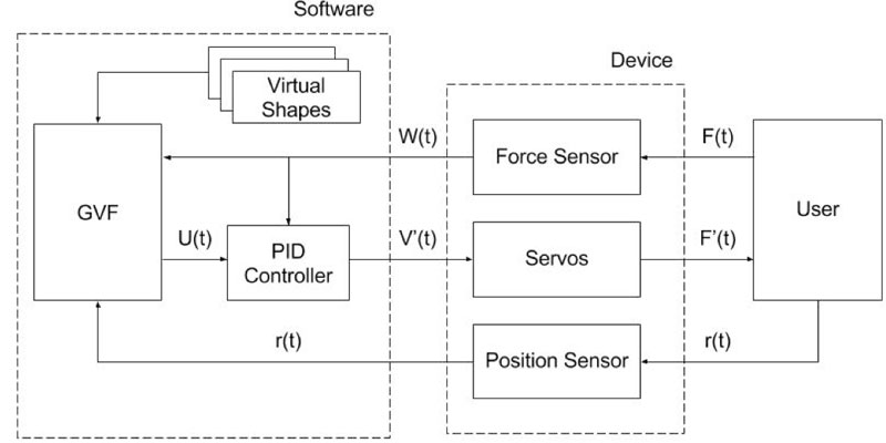
The system is divided into two main components. The first is the software which handles the virtual tactile diagram and the control of the device’s many features. The second part is the actual device hardware.
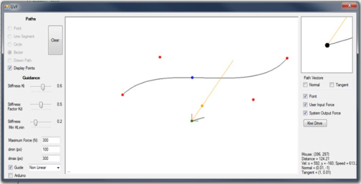
The software is further broken down into two modules. The first module handles the virtual tactile diagrams. It is programmed in C# using Visual Studio and runs on any desktop PC. Shapes (i.e., objects and parts) can be drawn or interpreted in the virtual workspace. Currently, the software interprets them as virtual fixtures. These fixtures produce virtual forces in response to user input force and position. To control the end result, an admittance control model of the type V = k * F is devised where F is the user input force and V is the system output velocity. Alternatively, path planning can be used to “forceably” guide the user explicitly through a path, such as around the edge of a shape. The System output is fed into the second software module designed to control and manage the device hardware. This second module was programmed in Arduino’s C++ and runs on an Arduino Due. The Arduino software is responsible for collecting and relaying input from the sensors in the device to the PC software and calculating the response of each actuator in the device.
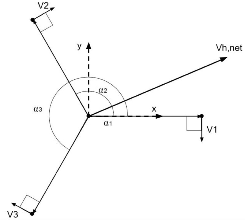
The final component of the system is the device hardware which consists of a 2D force sensor, RF position sensor and three servo motors as the actuators. As the user interacts with the device, the force sensor and position sensor collect the user’s intentions to move and relays the information to the software via the Arduino Due. Next the software determines a response and outputs a net velocity Vh,net through the use of the three servo motors.
Omni Drive Design
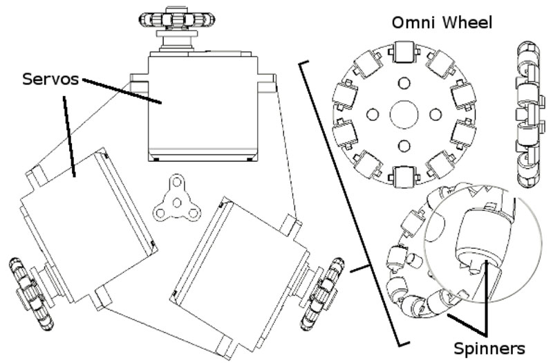
The three servo motors are concentrically positioned around the main vertical axis of the drive at 120° apart. This type of drive layout is known as a holonomic drive system. With the help of the omni wheels, this type of drive system allows for the control of all three degrees of freedom that the device has. The device can be linearly moved along the x and y axis and rotated around the z axis freely. Figure 2 below illustrates the design of both the holonomic drive system and the omni wheels respectively.
The device sensors consist of a 2D force sensor (MSI Model 462, Ultra-MSI) and a 2D RF position sensor that interfaces with a graphics tablet (Wacom Intuos Extra Large). Both sensors are housed in the device and are fastened on top of the drive platform. The force sensor specifically acts as a connector between the drive and the outer shell of the device. As the user applies a force to the outer shell, the force sensor will measure and relay it to the Arduino Due as an input force F for the admittance control model.
Guidance Virtual Fixtures
Virtual fixtures are forces and positions produced virtually that can be reapplied to an end manipulator for correcting or restricting movement. Guidance virtual fixtures (GVF) are a type of virtual fixtures that help to guide a human operator along a desired path. GVFs are categorized under two control models: impedance and admittance. An impedance model uses position and velocity as the input and outputs a force. This model is usually low in inertia and back drivable. An admittance model, in contrast, uses force and position as the input and outputs a velocity to the end effector. This model type helps to constrain the user’s movements to a given path or region. High inertia and non-back drivable actuators are typically used to enforce the desired stiffness (Abbott et al., 2007).
For the current application a pseudo-admittance model is used that primarily constrains a user’s movements to a path but do allow the user to “break free” to freely explore other areas of the diagram. Such “soft” haptic fixtures have previously been described by (Bowyer et al., 2007). The method allows our device to seamlessly adapt to both passive and active tactile exploration methods used with traditional tactile maps.
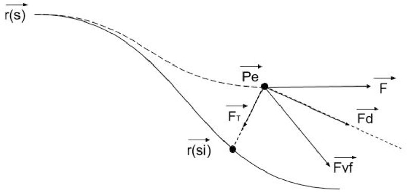
The main goal of the admittance GVF model is to respond to user input by encouraging desired motions, such as to follow a curve, and limiting undesired motions, such as moving away from a curve. The position of the end manipulator Pe is taken and used to calculate the closest point on the virtual path (curve) to the end manipulator.
With the closest point achieved, we can calculate the desired d and undesired τ direction unit vectors which are dependent on the position of the end manipulator Pe (see Figure 3). The two unit vectors are the tangent and normal vectors of the path at the closest point respectively. The input force F from the hand is projected onto the desired and undesired directions to produce the desired Fd and undesired Fτ forces of the user.
(1)
(2)
(3)
The admittance model uses an admittance variable ![]() to map the force to a final velocity (Bettini et al., 2004; Mihelj et al., 2012).
to map the force to a final velocity (Bettini et al., 2004; Mihelj et al., 2012).
(4)
Omni Drive Control Model
The omni drive of the device consists of three servo motors positioned concentrically 120° apart. To guide the user along a path on the virtual tactile diagram, the device’s drive module must take the commanded output velocity Vh,net (calculated through admittance control with virtual fixtures, as above) and decompose it into three distinct velocity components Vi = V1, V2, V3. More specifically the output for each servo is an angular velocity: (Tzafestas, 2014). Relating the wheel velocity components to the rotation of the motors:
(5)
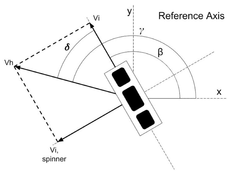
![]() , run along the radius of the main wheel frame. The spinners induce their own velocity Vi,spinner. Together the wheel velocity Vi and spinner velocity Vi,spinner produce a net velocity Vh which contributes to the final Vh,net. Vh is given:
, run along the radius of the main wheel frame. The spinners induce their own velocity Vi,spinner. Together the wheel velocity Vi and spinner velocity Vi,spinner produce a net velocity Vh which contributes to the final Vh,net. Vh is given:
(6)
As Figure 4 shows above, the resulting velocity of the omni wheel is denoted as Vh and is at an angle δ. Thus Vh can also be written as.
(7)
If we take into account the angle of Vh, shown as γ, in respect to the drive platform’s x axis and angle β which is the angle of the wheel’s linear velocity Vi in respect to the x axis, then we get δ = γ – β.
(8)
(9)
If we distribute Vh then we can get the x and y components of Vh as:
(10)
(11)
(12)
(13)
SOFTWARE TESTING
OUTCOME AND DISCUSSION
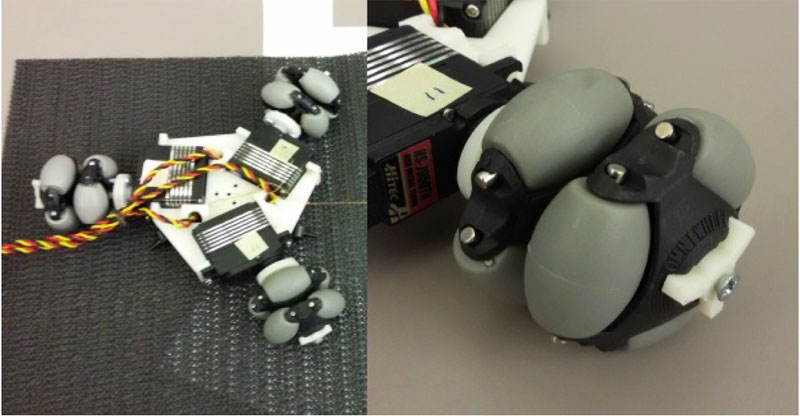
We have successfully developed an omni directional drive prototype. The Arduino Due C++ code allows for an input net velocity to be decomposed into three distinct velocities for each wheel in real-time. The device’s drive is thus capable of producing smooth 2D translations of various magnitudes. Currently the most significant limitation is a loss of traction of the wheels on a smooth surface. Preliminary tests show the device capable of producing 0.36 pounds of force in any given direction before the plastic omni wheels lose traction with the surface underneath. Figure 7 below shows the drive prototype and wheel design. Traction is improved by operating on a matted rubber toolbox liner.
FUTURE WORK
The current prototype is developed in two separate components. The virtual fixtures software is separate from the actual device drive system. Future work includes the merging of the two components into a cohesive real-time system that is responsive to user inputs. We are also working towards a custom wheel design to improve traction and to miniaturize the entire design. End user testing and further device performance assessment is planned for the future.
REFERENCES
Abbott, J. J., Marayong, P., & Okamura, A. M. (2007). Haptic Virtual Fixtures for Robot-Assisted Manipulation. Springer Tracts in Advanced Robotics Robotics Research, 49-64.
Abu Doush, I., Pontelli, E., Simon, D., Cao Son, T. and Ma, O. (2009). Making Microsoft Excel Accessible: Multimodal Presentation of Charts. ASSETS’09, Pittsburgh, PA, 147-154.
Bowyer, S. A., Davies, B. L., & Baena, F. R. (2014). Active Constraints/Virtual Fixtures: A Survey. IEEE Trans. Robot. IEEE Transactions on Robotics, 30(1), 138-157.
Gibson, J. J. (1962). Observations on active touch. Psychological Review, 69(6), 477-491.
Magee, L. E., & Kennedy, J. M. (1980). Exploring pictures tactually.Nature, 283(5744), 287-288.
Metec, AG. (2010). Braille cell P16. Retrieved September 27, 2011, from http://www.metecag.de/braille%20cell%20p16.html
Mihelj, M., & Podobnik, J. (2012). Haptics for Virtual Reality and Teleoperation (1st ed., Vol. 64, Intelligent Systems, Control and Automation: Science and Engineering). Springer Netherlands.
Owen J., Petro J., D’Souza S., Rastogi R., & Pawluk D.T.V. (2009). An Improved, Low-cost Tactile “Mouse” for Use by Individuals Who are Blind and Visually Impaired. Assets’ 09, October 25-28, Pittsburg, Pennsylvania, USA 2009.
Petit, G., Dufresne, A., Levesque, V., Hayward, V., & Trudeau, N. (2008). Refreshable Tactile Graphics Applied to Schoolbook Illustrations for Students with Visual Impairment. ASSETS 2008, 89-96.
Rastogi, R. and Pawluk, D. (2013a). Tactile DiagramSimplification on Refreshable Displays. Assistive Technology, 25 (1), 31-38.
Rastogi, R. and Pawluk, D. (2013b). Intuitive Tactile Zooming for Graphics Accessed by Individuals who are Blind and Visually Impaired. IEEE Transactions on Neural Systems and Rehabilitation Engineering, 21 (4), 655-663.
Symmons, M., Richardson, B., Wuillemin, D., & Vandoorn, G. (2005). Active versus Passive Touch in Three Dimensions. First Joint Eurohaptics Conference and Symposium on Haptic Interfaces for Virtual Environment and Teleoperator Systems.Tzafestas, S. G. (2014). Introduction To Mobile Robot Control (1st ed.). Waltham, MA: Elsevier.
Vermeij, G. J., Magee, L. E., & Kennedy, J. M. (1980). Exploring Pictures by Hand. Nature, 285, 59