Vladimir Kulyukin and John Nicholson
Assistive Technology Laboratory
Department of Computer Science
and
Center for Persons with Disabilities
Utah State University
Logan, UT 83422-4205
ABSTRACT
Modern GPS receivers are simple to operate, inexpensive, and commercially available. However, studies show that GPS-based localization has a great degree of inconsistency outdoors. The principal problem with GPS is signal drift, which may result in localization errors of up to 100 meters. This paper proposes a localization method that exploits the regularities in signal drift in a given area. The method is based on the observation that while the latitude and longitude for a given position drift over time, they tend to remain within a limited area. Successful localization experiments are presented.
KEYWORDS
Visual impairment, blindness, assisted navigation, outdoor localization, GPS.
BACKGROUND
 |
|---|
The 11.4 million visually impaired people in the United States continue to face a principal functional barrier: the inability to navigate [3]. Many wayfinding solutions that assist the visually impaired with outdoor navigation rely on the Global Positioning System (GPS) to determine a person's location [5]. The principal advantage of GPS is the commercial availability of inexpensive signal receivers that continuously output the latitude and longitude readings of their current location. When available, GPS signals can, theoretically, be used to localize their receivers within 3 to 5 meters of their true location.
 |
|---|
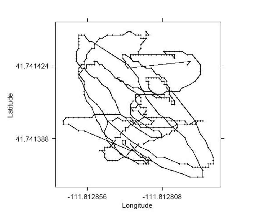
The principal problem with GPS is signal drift [1]. Even if the user stands still and receives multiple GPS readings from her receiver, the signal drifts over time. Such signal drifts can result in localization errors of up to 100 meters. Figure 1 shows the latitude and longitude drift at a landmark. Data were collected for ten minutes without moving the GPS unit at a location on the USU Campus. The points represent individual readings. The line represents the path of the drift. In addition, passing cars, tree cones, and tall buildings are known to cause single GPS readings to be significantly off the mark. Thus, associating a landmark with a single longitude-latitude GPS reading, which commercial street map software packages do, is error prone.
 |
|---|
HYPOTHESIS
It is hypothesized by the investigators that GPS-based outdoor localization can be improved by using regularities in signal drift in a given location. The hypothesis is based on the empirical observation that while the latitude and longitude for a given position drift over time, they tend to remain within a limited area.
METHOD
Instead of matching a single GPS reading to an actual position on the map, a virtual landmark is created based on the standard deviation of the drift. Specifically, standard deviation ellipses are computed for each selected landmark. Since, during navigation, single GPS readings are no longer mapped to single positions on the map, localization error is greatly reduced. Each location is associated with an ellipse based on the standard deviation of several readings taken at that location. To collect the data for the ellipses, 12 positions were identified on the Main USU Campus quad, a 2080 square meter area (See Figure 2). All 12 positions are located on the two orthogonal sidewalks. Each position is located 3 meters from a turn, which allows for sufficient time to give an advanced warning to the user about a turn. At each position, two sets of readings are taken: one on each side of the sidewalk. These two sets are combined into one large set of readings which are used to create the standard deviation ellipses. Since the readings are on each side of the sidewalk, the ellipse covers the entire area between the two points, creating the virtual position through which the user will walk with a GPS receiver.
The GPS receiver used for data collection is a TripNav™ TN-200 receiver from the the Rayming Corporation. It connects to a computer via USB and there are USB-to-serial drivers for both Linux and Windows. To send data, the GPS receiver uses the National Marine Electronics Association (NMEA) protocol NMEA-0183. GPS readings were obtained at a rate of approximately one reading per second. The GPS unit was placed at each side location on both sides of the sidewalk for ten minutes at a time. This was repeated six times for each spot, resulting in one hour of data for each side of the sidewalk, or two hours of total data for each position. A total of six days were required to collect the data for each position.
Once the data collection was completed, the standard deviation ellipses were computed using dispersion point pattern techniques [2]. First, the mean center is calculated. The mean center for a collection of N coordinates is the X-Y coordinate, where X is the average of the longitudinal readings and Y is the average of the latitudinal readings. To reflect the true spread of the data, a rotated ellipse is used. The ellipse is rotated around the mean center with the long axis representing the direction of maximum dispersion and the short axis representing the direction of minimum dispersion. As defined in Equation 1, the ellipse's angle of rotation, Θ (theta), represents the angle in a clockwise direction from the y axis. The standard deviations along the x-axis of the ellipse, σ x (sigma sub x), and the y axis of the ellipse, σ y (sigma sub y), are calculated using Levine’s formula [3] given in Equation 2.
Equation 1: 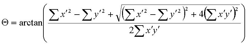
Equation 2: 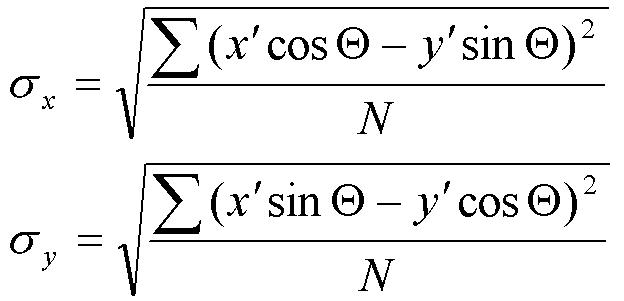
RESULTS
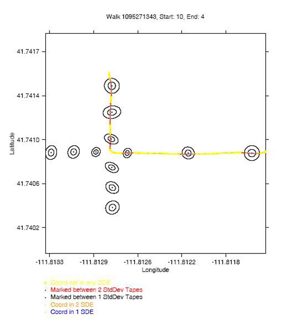
The method was tested using the 12 positions on the Main Quad of the USU Campus (See Figures 2 and 3.) For each position the maximum distance east, west, north, and south from the mean center was calculated using the first and second standard deviation ellipses for each position. The distances were then marked from the position where the data was originally collected. Only the distances for each position's appropriate direction were marked. This resulted in four markings for each position.
Two users then walked several routes through the marked area. Each user walked five different routes, 3 straight routes and 2 routes with a turn. When the user passed over a distance marking for a given position, they pressed a button to indicate that they had passed over the marking. This allowed the system to save the fact that they were between the 2 markings for the second standard deviation distance and also between the 2 markings for the first standard deviation distance. The collected data were processed off-line so that each GPS reading was evaluated to determine if it was inside a standard deviation ellipse. A sample plot is shown in Figure 3. A total of 10 walks were performed with each walk passing through six ellipses. An intersection was defined as at least one GPS coordinate being inside an ellipse. Out of a total of 60 possible intersections with the set of second standard deviation ellipses, there were 60 intersections total, or 100% correct intersections. The walk paths intersected with 54 out of the 60 first standard deviational ellipses, an accuracy of 90%. While several of the paths missed the first standard deviation ellipses, all of them succeeded in intersecting with the second standard deviation ellipses.
DISCUSSION
The investigators were encouraged by these results. Work is under way to reduce the amount of data collection at each location to approximately 2 minutes.
REFERENCES
- Abowd, G., Mynatt, E. (2000). Charting Past, Present, and Future Research in Ubiquitous Computing. ACM Transactions on Computer-Human Interaction, 1(7), 29-58.
- Edbon, D. (1985). Statistics in Geography. (2 nd ed.). London, England: Basil Blackwell.
- LaPlante, M. P. & Carlson, D. (2000). Disability in the United States: Prevalence and Causes. Washington, DC: U.S. Department of Education.
- Levine, N. (2002). A Spatial Statistics Program for the Analysis of Crime Incident Locations. Washington, DC: National Institute of Justice.
- http://www.senderogroup.com/gpsflyer.htm. “What is GPS-Talk?” Sendero Group, LLC.
ACKNOWLEDGMENTS
The study was funded by two Community University Research Initiative (CURI) grants from the State of Utah (2003-04 and 2004-05) and NSF Grant IIS-0346880. The authors would like to thank Mr. Sachin Pavithran, a visually impaired training and development specialist at the USU Center for Persons with Disabilities, for his feedback on the localization experiments.
Author Contact Information:
Vladimir Kulyukin, Ph.D.
Assistive Technology Laboratory
Department of Computer Science
Utah State University
4205 Old Main Hill
Logan, UT 84322-4205
Office Phone (435) 797-8163
EMAIL: vladimir.kulyukin@usu.edu.